Crimecouver

October 23 2017

Visualizing crime data with Mapbox GL JS and React

This short tutorial describes how I collected, managed, and visualized the City of Vancouver's crime data using React as well as Mapbox Studio and GL JS. I conducted this project as a way to learn React, so this tutorial is catered towards those who know the basics of React; but, as the code is relatively simple, it can be understood by beginners. The code is accessible here.

In 2017, the City of Vancouver released new crime data on their open data catalogue. As I wanted to learn React and I saw no pre-existing interactive data visualizations on Vancouver crime, this was a perfect opprotunity to develop an interactive map to learn React with Mapbox GL JS. The following discusses how I collected, managed, and visualized the data.

Data Collection

I wanted to incorporate an interactive map into the data visualization, so I downloaded data that was explicitly georeferenced with coordinates.

City of Vancouver: crime data 2003-2016 (14 shapefiles: crime_shp_[year].shp), local area boundaries (local_area_boundaries.shp), and parks (parks_shp.shp).
OpenStreetMap

After downloading crime_shp, I reviewed the metadata to help brainstorm how I would visualize the data on an interactive map.

crime_shp stored geographic points with the following attributes/properties: neighbourhood of the crime, type of crime, address of the crime (without the address number to maintain privacy), year of crime, month of crime, day of crime, hour of crime, and minute of crime.

With these attributes, I wanted to incorporate filters by year and type of crime. I also wanted practice developing a choropleth map with Mapbox GL JS, so I decided that I would calculate the total amount of crime by neighbourhood. I needed the geograhpic locations of the Vancouver neighbourhoods, so I downloaded local_area_boundaries.

local_area_boundaries stored polygons with the geographic coordinates and names of each neighbourhood in Vancouver. I also downloaded parks_shp because local_area_boundaries did not include Stanley Park, which was considered a neighbourhood in crime_shp.

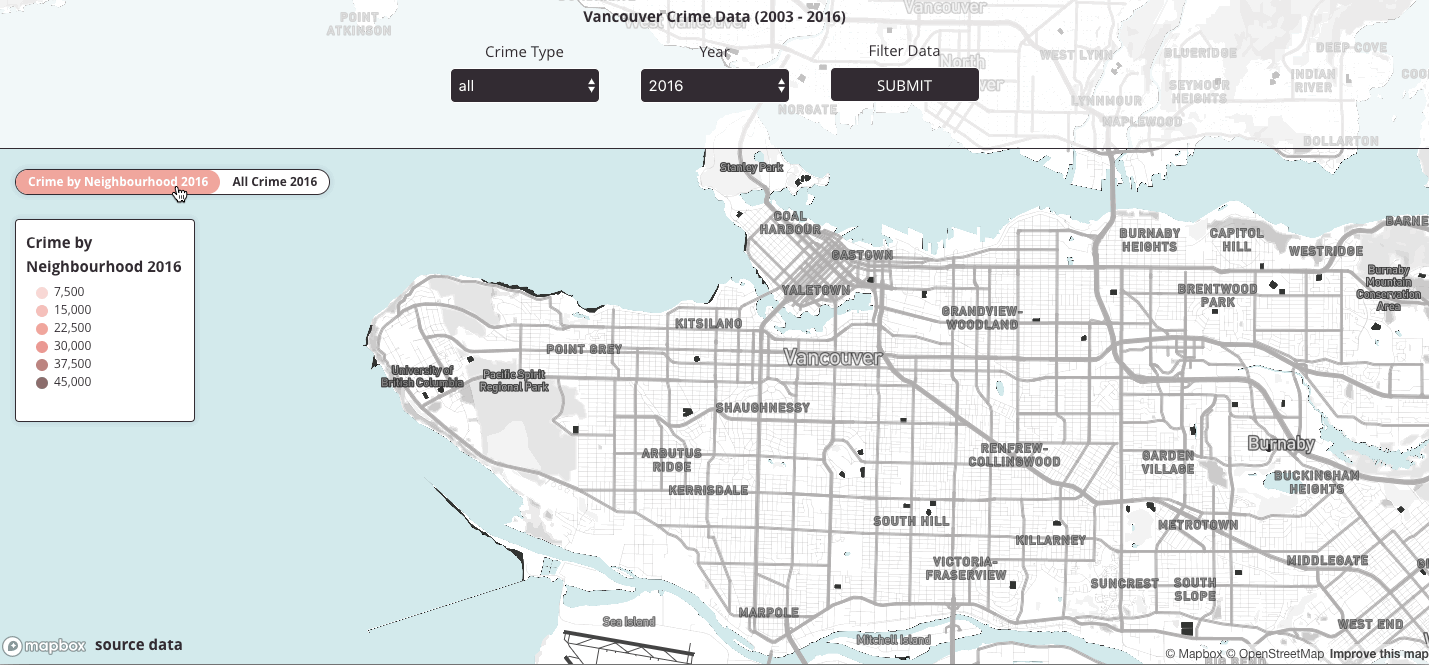
After brainstorming and sketching, I had a general gist of how I wanted to develop the interactive map. I wanted users to have the ability to control the year and type of crime visible on the map. I also wanted users to see a choropleth map of the most recent, 2016, crime data count by Vancouver neighbourhood. With this in mind, I decided to develop the interactive map as the focal point and then add a side panel to store the filters users could interact with.

I certainly have other plans to visualize the data; for example, since the metadata stores the date of the crime, I would like to visualize with a time slider the relation between time and type of crime.

Data Management

For the crime data 2003-2016, I originally downloaded the JSON because I prefer to handle the data as a GeoJSON, but I had a difficult time converting the JSON’s projection on QGIS and ogr2ogr; so, instead I downloaded all the shapefiles. Basically when I tried to convert the JSON into a GeoJSON using the '... Save as' method on QGIS, the GeoJSON would state the CRS was EPSG 4362: WGS 84, but the coordinates were in meters, not decimal degrees.

To avoid repeating each step for each shapefile, I merged all the shapefiles into one shapefile. I used this ogr2ogr line. In Terminal (I use a Mac) I entered the following command that creates a new merge file from the first shapefile:

ogr2ogr -f ‘ESRI Shapefile’ merge.shp crime_shp_2003.shp

With a new merge shapefile (merge), I then ran the following script for every shapefile (crime_shp_2004.shp, crime_shp_2005.shp...) I wanted to merge to the merge shapefile:

ogr2ogr -f ‘ESRI Shapefile’ -update -append merge.shp [crime_shp_year.shp].shp -nln merge

I initially wanted to use QGIS's merge data management tool, but it took 3 hours to complete only 50% of the process. When I tried the ogr2ogr method in Terminal, it took ~ 2 minutes.

With the merged shapefile, I then had to convert the shapefile into a GeoJSON so that I could then use tippecanoe to convert the GeoJSON into MBTiles. I used MBTiles over a GeoJSON because MBTiles converted the GeoJSON into a tileset which, in general, renders more easily.

I converted the shapefile into a GeoJSON in QGIS. All you have to do is click '... Save as' and then select the file type (GeoJSON), the location of where to save the GeoJSON, and then the geographic coordinate sytem. The standard for MBTiles is EPSG 4362: WGS 84, so I made sure my GeoJSON was in that format.

Once I had the GeoJSON (vancouver_crime), I then used tippecanoe in Terminal:

tippecanoe --layer vancouver_crime -o vancouver_crime.mbtiles --minimum-zoom=11 --maximum-zoom=20 < vancouver_crime.geojson

My output was a MBTile file (vancouver_crime.mbtiles) that stored all the crime vector points from 2003 to 2016.

The next step was to create the data for the choropleth map. To accomplish this I used QGIS. First I had to merge local_area_boundaries with a polygon of Stanley Park. I extracted the Stanley Park vector polygon from parks_shp by using the Filter tool ("NAME" = "STANLEY PARK") and then saving the output as a new layer. Then I used Vector > Data Management Tools > Merge Vector Layers to merge the Stanley Park extracted polygon to local_area_boundaries. Lastly, I used the Vector > Data Management Tools > Join Attribute by Location tool to calculate basic statistics, including the crime count, within each neighbourhood boundary. My inputs for the 'Join Attribute by Location' were the vancouver_crime GeoJSON and local_area_boundaries.

Once I had the statistical crime data (count, mean, mode, median) for each neighbourhood represented in vancouver_crime, I followed the same steps as above to convert the shapefile into MBTiles (vancouver-crime-nhoods.mbtiles).

Data Visualization

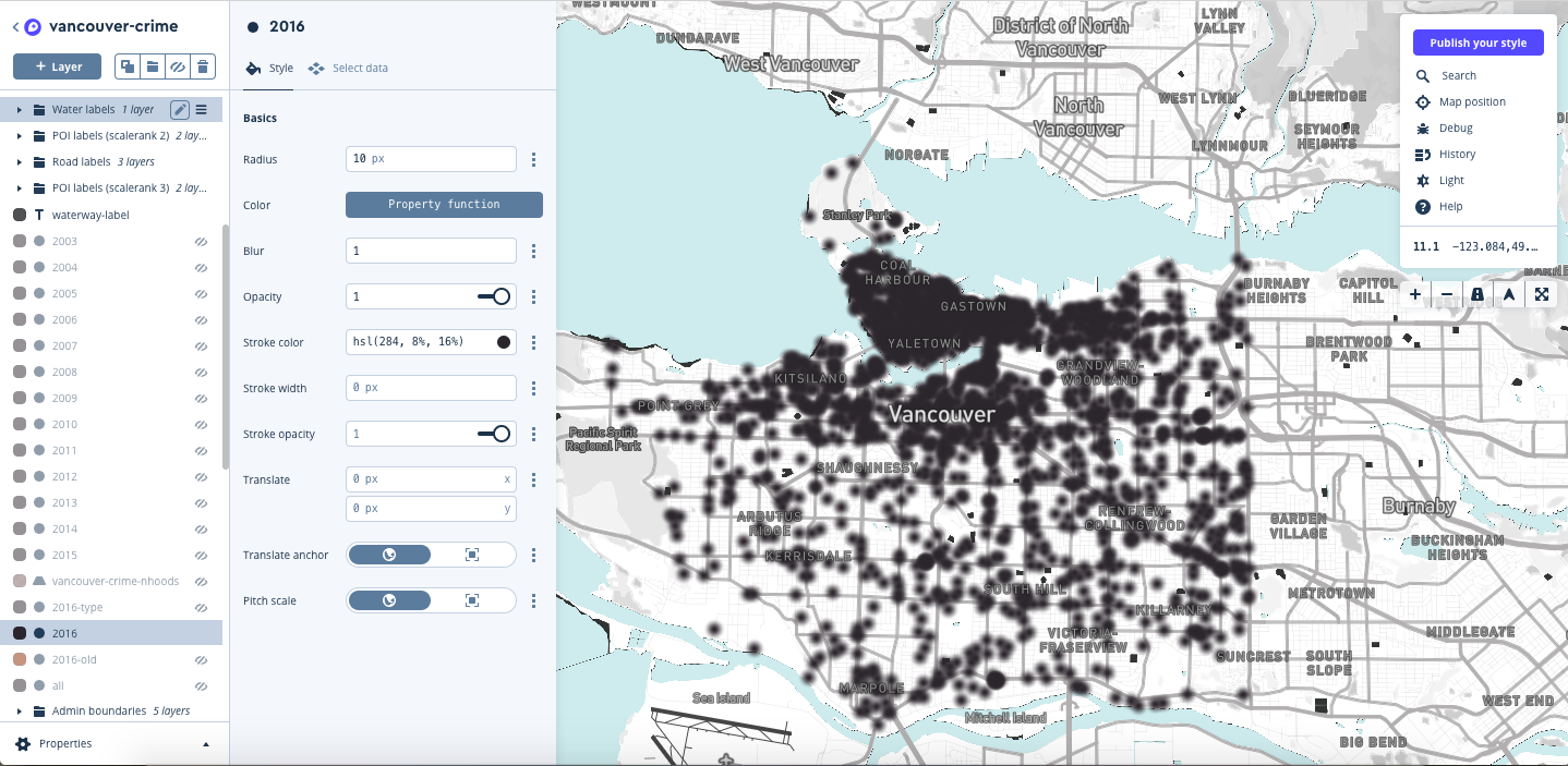
To avoid slowing the browser with too much JavaScript, I decided to import the MBTiles (vancouver_crime.mbtiles and vancouver-crime-nhoods.mbtiles) into Mapbox Studio and then use Mapbox GL JS to interact with my custom style layer's data.

In Mapbox Studio, I imported vancouver_crime.mbtiles as a new layer on my custom map style and then I created new layers from the vancouver_crime layer by filtering the data by year. Basically, I create a layer of crime data by each year between 2003 and 2016.

After creating and designing all the layers, the next step was to import my custom map style into React, so I published the Mapbox style and copied the token and then I reviewed examples in the Mapbox react-examples repo and POI blog post. This source was useful to develop React infrastructure necessary to use Mapbox GL JS with React.

import React from 'react'
import ReactDOM from 'react-dom'
import mapboxgl from 'mapbox-gl'

class Application extends React.Component {
	constructor(props: Props) { ... }
	componentDidUpdate() { ... }
	componentDidMount() { ... }
	render() { 
		return ( ... );
	}
}

ReactDOM.render(<Application />, document.getElementById('app'));

I then used this code as a frame (index.js) to develop the interactive map.

I first added the map to componentDidMount():

this.map = new mapboxgl.Map({
	container: this.mapContainer,
	style: 'mapbox://styles/julconz/cj7rpgkw4e3yl2smwad8ddg7c',
	center: [-123.1846069, 49.265],
	zoom: 11.7,
	maxZoom: 18,
	minZoom: 11
});

Then in return() I added the map container to store the map:

<div ref={el => this.mapContainer = el} className="absolute top right left bottom" />

With a rendered map, the next step was to develop the interactive components for the map. More specifically, I coded with Mapbox GL JS and React to develop drop-drown menus and a submit button that allows users to select and submit what data appears on the map.

First, I declared two new variables years and types that each stored the information necessary to develop the filters. years stores the data's years of crime (2003-2016) so that users can filter data by year. types stores the name and value of the crime types so that a user could filter data by type of crime. The following shows an example of how I declared the variables:

const years = [{name: 'all'}, {name: '2016'}, {name: '2015'}, ... {name: '2003'}];
const types = [{name: 'all', value: 'all'}, ... {name: 'Other Theft', value: 'Other Theft'} ... ];

To create the two drop-down menus, I added to function in render():

const renderYears = (years, i) => {
	return (
		<option key={i} value={years.name}>{years.name}</option>
	);
}

const renderTypes = (types, i) => {
	return (
		<option key={i} value={types.value}>{types.name}</option>
	);
}

Then in return() I added the following:

<div className="filters">
	<form onClick={this.handleSubmit.bind(this)}>
		<div className="filter-container">
			<label>Crime Type</label>
			<select name="type" className="filter" id="types" 
			value={this.state.selectValues["type"]} onChange={this.handleChange.bind(this)}>
				{types.map(renderTypes)}
			</select>
		</div>
		<div className="filter-container">
			<label>Year</label>
			<select name="year" className="filter" id="years" 
			value={this.state.selectValues["year"]} onChange={this.handleChange.bind(this)}>
				{years.map(renderYears)}
			</select>
		</div>
		<div className="filter-container" >
			<label>Filter Data</label>
			<input id="submit" type="submit" value="SUBMIT" />
		</div>
	</form>
	<div id="stats" className="txt-bold"></div>
</div>

Basically renderYears runs through all objects in years and renderTypes runs through all objects in types to each create a drop-down menu. Now with the filters developed to render, the next step was including the onClick function after users click the submit button. Above, you can see I added onClick in the form tag:

  handleSubmit(event) {
    event.preventDefault();

    this.map.setLayoutProperty('2016', 'visibility', 'none');
    
    // input the selected values
    this.setFilter(this.state.selectValues); 
    this.setStats(this.state.selectValues);
  }

So onClick runs setFilter() and setStats():

setFilter(values){
	var filter = [];

	// hide legend & toggle if it is not 2016 data
	if (values.year !== '2016'){
		document.getElementById('legend-choropleth').style.display = 'none';
		document.getElementById('toggle').style.display = 'none';
		this.map.setLayoutProperty('vancouver-crime-nhoods', 'visibility', 'none');
	}

	// based on selection, output the following filter
	if (values.type !== 'all' && values.year !== 'all'){
		filter = ['all', ['==', 'TYPE', values.type], ['==', 'YEAR', parseInt(values.year)]];
	} else if (values.year === 'all' && values.type !== 'all') {
		filter = ['==', 'TYPE', values.type];
	} else if (values.year !== 'all' && values.type === 'all') {
		filter = ['==', 'YEAR', parseInt(values.year)];
	}

	// apply the filter and then make the layer visible on the map
	this.map.setFilter(values.year, filter)
	this.map.setLayoutProperty(values.year, 'visibility', 'visible');
}

setStats(values){
    // need to figure out how to get all data from layer, not just what is rendered
    //var features = this.map.queryRenderedFeatures({layers:[values.year]});

    if (values.type === 'Vehicle Collision or Pedestrian Struck (with Injur') {
      values.type = 'Vehicle Collision or Pedestrian Struck (with Injury)';
    }

    if (values.type === 'Vehicle Collision or Pedestrian Struck (with Fatal') {
      values.type = 'Vehicle Collision or Pedestrian Struck (with Fatality)';
    }

    if (values.year === 'all'){
      values.year = 'all years';
    }

    document.getElementById('stats').innerHTML =  values.type + " in " + values.year;
 }

setFilter() adjusts the data on the map based on the year and crime type the user selects, while setStats() outputs in text what the user selected by filter. Overtime I will actually add statistical information to setStats(), but I still need to figure out how to access all the data points from the layer because currently the functions available on Mapbox GL JS can only give the amount of points rendered on the map.

With the above code, a user should be able to select the crime year and type, click submit and then see filtered data appear on the map. Next I will show how I incorporated the choropleth map.

Since I decided to only have a choropleth for 2016 data, I added a toggle function that would only be visible when the 2016 year is selected. First, I declared the toggle options (i.e., what layers can be toggled to appear on the map):

const options = [{
	name: 'Crime by Neighbourhood 2016',
	layer: 'vancouver-crime-nhoods',
	otherLayer: '2016',
	stops: stops},
	{name: 'All Crime 2016',
	layer: '2016',
	otherLayer: 'vancouver-crime-nhoods',
	stops: []
}]

The information includes the name of the data, the name of the data layer stored in my custom Mapbox style, and the stops (i.e., the colours and count value) that will populate the choropleth legend if selected. Now, I had to create the toggle function and legend, so in return() I added the following:

// toggle
<div id="toggle" className="legend toggle-group border border--1 shadow-darken10 z1">
	{options.map(renderToggle)}
</div>

// choropleth legend
<div id="legend-choropleth" className="legend absolute top left shadow-darken10 round wmax180">
	<h2 className="txt-bold block">{name}</h2>
	{stops.map(renderLegendKeys)}
	<p className="txt-bold block" id="stats-choropleth"></p>
</div>

I then created a function in render() to run through options and create the toggle function options and choropleth legend:

const renderToggle = (option, i) => {
	return (
		<label key={i} className="toggle-container">
			<input onChange={() => this.setState({ active: options[i] })} 
			checked={option.layer === layer} name="toggle" type="radio" />
			<div className="toggle txt-s py3">{option.name}</div>
		</label>
	);
}

const renderLegendKeys = (stop, i) => {
	if (stop.length){  
		return (
			<div key={i} className='txt-s'>
				<span className='mr6 round-full w12 h12 inline-block align-middle' style={{ backgroundColor: stop[1] }} />
				<span>{`${stop[0].toLocaleString()}`}</span>
			</div>
		);
	}
}

Lastly, none of the above code would work unless I added a function for when the toggle was changed by users:

handleToggle(event) {
	let layer = this.state.active.layer;
	let otherLayer = this.state.active.otherLayer;

	this.map.setLayoutProperty(otherLayer, 'visibility', 'none');
	this.map.setLayoutProperty(layer, 'visibility', 'visible');
}

... and in handleToggle(event):

componentDidUpdate() {
	this.handleToggle();
}

At this point, the interactive map should now have filters that allow users to select both the year and type of data to be visible on the map; in addition, the user has the option to select a choropleth map if they select the year 2016. Additional functionalities, such as popups, can be seen in the final code, which is accessible here.