Literature Review
Since the widespread use of OSM, academics have published an array of peer-reviewed articles that assess the quality of OSM data. Although academics have applied various formulas at varying complexities to assess the quality of OSM nodes, ways or polygons, most academics approach the assessment through comparing a reference dataset (e.g., a government dataset), which is considered to be an accurate, authoritarian, dataset, with an OSM dataset.
With this approach, most research initially focused on comparing the quality of OSM ways/lines, such as roads or road networks, with a reference dataset (Haklay 2010; Ludwig et al. 2011; Zielstra and Zipf 2010; Neis et al. 2011). For instance, Haklay (2010) was one of the first academics to assess OSM quality by comparing the geometric positions of roads in OSM to roads in United Kingdom’s Ordnance Survey (OS). He accomplished this by applying buffers around the OS’s roads and then computing whether the OSM roads fit within the buffer. That said, more recently academics have evaluated the quality of OSM buildings as well (Girres and Touya 2010; Hecht et al. 2013; Fan and Zipf 2014; Brovelli et al. 2016; Müller et al. 2015).
Although comparing datasets has become a de facto methodology, sometimes a reference dataset may be inaccessible due to high costs or unavailable as no data exists; moreover, if the only authoritative dataset for a given region has already been imported onto OSM, it then cannot be used as a reference dataset. With this in mind, current research has pitched alternative approaches for assessing the quality of OSM data that do not require a reference dataset (Ciepluch et al. 2011; Sehra et al. 2017). For instance, Ciepluch et al. (2011) overlaid a grid of cells to calculate the number of OSM nodes per cell to ultimately assess OSM coverage and concentrations of contributions within a given region. In another case, Ciepluch et al. suggests assessing the completeness of an OSM dataset at the “compound feature level,” such as determining whether all necessary tags for a given “compound polygon” exist (e.g., does a hospital have all the necessary tags present?). However, these approaches tend to be more qualitative in nature than quantitative (e.g., we may all have different perceptions of what tags should be associated with a hospital).
From the literature, the following are applied metrics to assess the quality of a given OSM dataset: lineage, completeness, positional accuracy, temporal quality, logical consistency, semantic accuracy, attribute accuracy, shape accuracy, and size accuracy (Haklay 2010; Fan and Zipf 2014; Girres and Touya 2010). For assessing OSM buildings specifically, literature originally focused on just assessing the completeness, but more research has been applied on matching buildings from an OSM dataset with buildings from a reference dataset and then assessing the positional, semantic, attribute, shape, and size accuracies (Brovelli et al. 2016).
The rest of this literature review will detail these metrics. Before continuing, however, another point in the literature is worth highlighting, mainly the idea of “fitness-for-purpose.” Quality of a dataset can be determined by its usage, or its “fitness-for-purpose” (Haklay 2010). This is important to consider because the quality of OSM data depends on how the data will be used. For instance, if one is assessing the average height of buildings in Ottawa, the positional accuracy of an OSM building footprint can be considered “great quality” if the difference between where the building actually exists on the ground is within 5 meters; but, a 5 meter difference may not be considered “great” if the data is needed for construction purposes. This approach to determining data quality should be kept in mind when conducting quality assessments.
Lineage
Lineage focuses on the history of the dataset, such as how the data was collected. This reflects on the process involved in developing the OSM data. For example, who contributed the data; was it a small group of experts contributing the data or a large group of inexperienced contributors?
Completeness
In general, completeness assesses “the presence or absence of features, their attributes and relationships;” but, for OSM data, completeness is usually measured by the absence of OSM features (e.g., nodes, ways, polygons) to a reference dataset (Hecht et al. 2013). For example, Hopfner (2011) evaluated the completeness of OSM polygons within a given area by calculating the total number of OSM addresses compared to the total number of reference addresses.
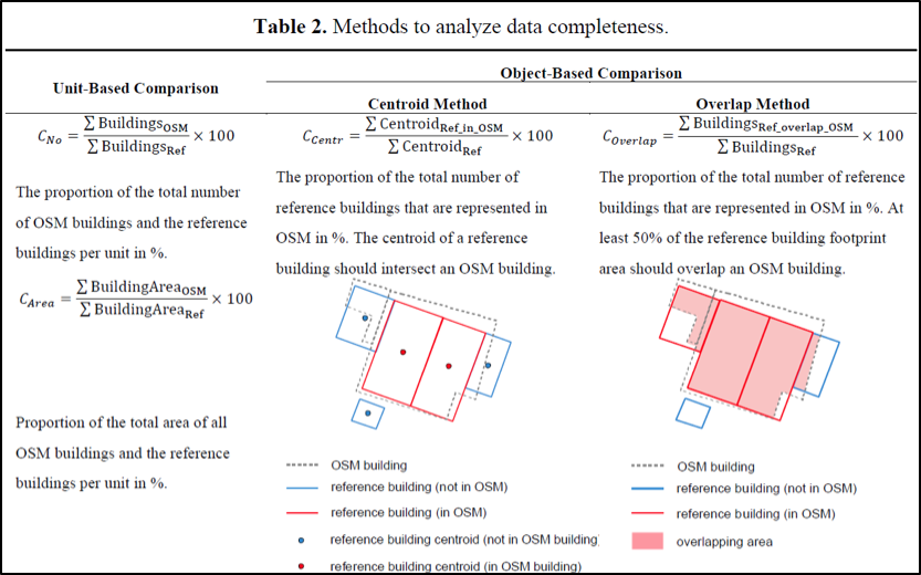
Hechet et al. (2013) introduced two dimensions to measure the completeness: “unit-based comparison” and “object-based comparison”.
Unit-based Comparison:
The unit-based comparison generally compares total features between an OSM dataset and a reference dataset. This dimension can assess both geometric (e.g., area) and attribute (e.g., address tags) features, but Hechet et al. focused their research on just the geometric features because there is not enough OSM attributes to assess. The attribute completeness is measured through calculating the total number of tags of a specific attribute (e.g., address) for each dataset and then measuring the proportion of the OSM total to the reference total. Similarly, to assess the geometric completeness, the total building count and total building area is calculated for each dataset and then the proportions are measured for both sets of totals (view Figure 2). Measurements are expressed as a ratio or percentage.
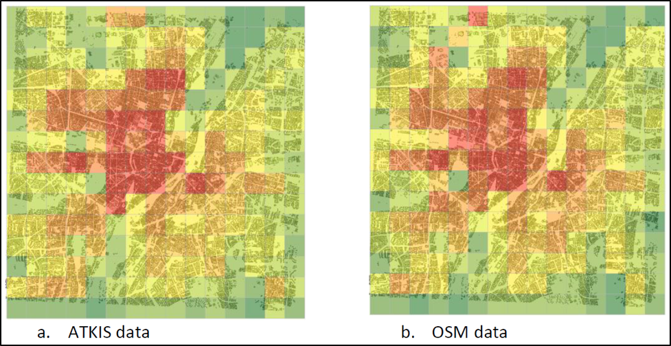
Fan and Zipf (2014) calculated the total building area between ATKIS data (their reference dataset) and OSM data. Then, following a widely adopted approach, they also applied a grid layer of cells over top of each dataset layer to calculate the total area of all buildings within each cell (view Figure 3; Haklay et al. 2011; Ciepluch et al.; Fan and Zipf 2014). This method can visualize the coverage to identify which regions within a given area are more complete over other regions. In Figure 3, for example, the city center is more complete than the rural areas.
The unit-based comparison is simple to apply, but it only provides a rough estimate of completeness because the level of detail is limited. This can result in over- or under-estimations of completeness (Hechet et al. 2013).
Object-based Comparison:
As for object-based comparison, this assesses completeness by matching the OSM buildings to reference buildings, either by centroid or area overlap, and then measuring the total number of reference buildings that match an OSM building over the total number of reference buildings (view Figure 2). Overall, this approach is more complex because of the necessary matching, but errors in estimations are reduced. This approach closely aligns with semantic accuracy, so refer to the “General Steps for Quality Assessment of OSM Building Data” section for details on how to match buildings between two datasets.
Positional Accuracy
The positional accuracy assesses whether or not a given OSM building is in the same coordinate location as it is on the ground (Haklay 2010). Depending on the intent of the data, this can be assessed at varying complexities. Simply, you can calculate the distance between an OSM building’s centroid and a reference building’s centroid. Alternatively, instead of comparing the distance of just one point in the center of both the buildings, you can assess the distance between multiple nodes along the edges of each building (Fan and Zipf 2014).
Temporal Quality
The temporal quality measures the quality of a dataset based on how up to date it is.
Logical Consistency
Logical consistency evaluates how consistent the data is organized internally. For instance, are all Tim Hortons in Ottawa registered as a “fast food” point-of-interest (POI), which would be considered logically consistent, or are some registered as “fast food” and others as “coffee shop”?
Semantic Accuracy
In general, semantic accuracy assesses whether an OSM object actually represents what is on the ground. Fan and Zipf (2014) measure this by matching buildings from the OSM dataset to buildings from the reference dataset. Matching can be accomplished in various ways, which is discussed more in the “General Steps for Quality Assessment of OSM Building Data” section below.
The matching methodology will determine whether an OSM building matches none, one, or many building(s) in the reference dataset. In other words, if comparing OSM:reference, there can be a 1:1, 1:0, 0:1, 1:n, n:1, or n:m relationship. With these relations, the semantic accuracy can be assessed. A 1:1 relation (i.e., 1 building from the OSM dataset matches 1 building from the reference dataset), then the OSM building is semantically correct.
If there is a 1:0 or 0:1, then a building in the OSM dataset is not a building, or a building in the reference dataset is not a building. Assuming the OSM dataset is more recent than the reference dataset, if there is a 1:0 relation, it is also considered semantically correct because the reference dataset may not include new buildings that the OSM dataset has. However, assuming the OSM dataset is more out-dated than the reference dataset, a 0:1 relation may also be semantically correct; for instance, a building in the reference dataset may not exist in the OSM dataset because the building was demolished. In either case, it is important to consider manually validating the 0:1 or 1:0 relations.
If there is a 1:n, then one building from the OSM dataset matches multiple buildings from the reference dataset, which indicates the building is recorded at a higher semantic level. n:1 relationship indicates that multiple buildings from the OSM dataset matches one building from the reference dataset, which indicates that the OSM building is recorded at a lower level on the semantic hierarchy. Lastly, n:m indicates that multiple buildings in the OSM dataset matches multiple buildings in the reference dataset, which indicates both buildings could be semantically incorrect.
Overall, relations 1:n, n:1, or n:m will always be semantically incorrect. So, to calculate the semantic accuracy, it is the percentage of 1:1 relations + (verified 1:0 relations or verified 0:1 relations) compared to all polygons that exist within the OSM dataset.
Note: The remainder of the metrics can be evaluated for the 1:1 relations.
Attribute Accuracy
Attribute accuracy determines whether an OSM object has accurate tagged attributes. For instance, is an OSM building tagged as “commercial” really commercial?
To measure the attribute accuracy, the matched OSM building’s attributes are compared to matched reference building’s attributes. Very few studies have compared building attributes between an OSM dataset and reference dataset because usually the OSM data has too few attributes (i.e., low completeness) to properly assess (Fan and Zipf 2014).
Shape Accuracy
Shape accuracy evaluates the shape of an OSM building relative to the on the ground shape. This is the most difficult metric to assess and it can be measured at varying levels of complexity. Depending on the intended use of the data, a different level of complexity can be considered. That said, there are two general trends for assessing the shape of a polygon: calculating the compactness ratio (Girres and Touya 2010; Li et al. 2013) or calculating the turning function (Fan and Zipf 2014; Mooney et al. 2010). In general, the former assesses shape by the degree of compactness, while the latter assesses shape through the tangent angles of a polygon`s vertices.
Compactness Ratio:
The compactness ratio originated from Miller (1953), but MacEachren (1985) applied the formula for shape comparison. Various research has applied the compactness ratio, but many have adjusted it. For example, the IPQ (Osserman 1978) considers the area and perimeter of a polygon to assess shape, while the Digital Compactness Measure (DCM) compares a polygon’s area with the “smallest circle that circumscribes the shape” (Li et al. 2013, 4). On the other hand, the shape can also be assessed through rasterizing the polygons and using the Normalized Discrete Compactness (NDC) measure that, in general, counts the number of cell sides that are shared between all pixels that denote a single polygon (ibid.).
Li et al. (2013) assessed how “robust”, "computationally efficient”, and “additive” the IPQ and NDC formulas were compared to their own Moment of Inertia (MIT) formula (3). After their comparison, Li et al. conclude the MIT formula is the most reliable because it can handle both vector and raster data, it is “insensitive to positioning errors,” seems to be consistent over varying scales, and can handle shapes that have holes and shapes that have irregular boundaries. That said, the MIT formula is relatively new and lacks an “efficient, computationally simple method of computing the moment of inertia” (25). With this in mind, determining which compactness ratio to apply involves trade-offs (e.g., computational efficiency over handling shapes with holes). For greater detail on each formula, refer to Li et al. (2013) article.
Turning Function:
Fan and Zipf (2014) and Mooney et al. (2010) assessed the shape accuracy of OSM buildings using the turning function, or tangent function, which originated from Arkin et al. (1991). This approach assesses the shape of polygons not by its vertices or edges, but by its turning functions; in other words, by “a list of angle-length pairs, whereby the angle at a vertex is accumulated tangent angle at this point while the corresponding length is the normalized accumulated length of the polygon sides up to this point” (Fan and Zipf 2014, 705). Then, to assess the similarity of a polygon (e.g., OSM building) to another polygon (e.g., reference building), the distance is calculated between the two polygons’ turning functions. The smaller the distance, the more similar the polygons are. Calculations are invariant to orientation and scale (because of the normalization of the length being independent of a polygon’s size).
Essentially, to calculate the turning function, Tc(l), for each polygon for a given dataset (e.g., the OSM dataset), the turning, or tangent, angle is calculated for each polygon’s vertices. The first tangent angle, at the first vertex, is 1 = 1. Then, moving counter-clockwise, i = i-1 + i…
As mentioned above, comparing an OSM building’s shape to a reference building’s shape is only done when there is a 1:1 relation, meaning these two buildings are matched, the building on OSM is the same building that in the reference dataset. However, these matched polygons may not have the exact same geometric position; so, to avoid translation affecting the turning function results, the two matched polygons’ initial vertex to assess should be matched as well. Fan and Zipf detail how to “find identical points of matched building footprint pairs” in Section 4.2 of their paper.
Once the turning functions are calculated for all the polygons in each dataset, the distance is calculated from the two polygons’ turning functions to identify how dissimilar the polygons’ shapes are. This is accomplished through the following formula (Fan and Zipf 2014):
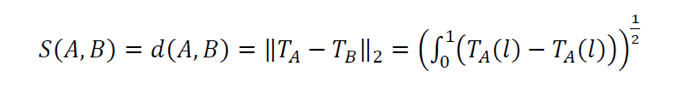
S(A,B) indicates the dissimilarly of two polygons, so the smaller the distance between the two polygons’ turning functions indicates that the polygons are more similar.
Size Accuracy
Lastly, size accuracy measures the size of an OSM building relative to the size of the on the ground building. This can be accomplished through comparing the normalized area and perimeter between an OSM polygon and reference polygon (Fan and Zipf 2014):
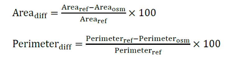
The area and perimeter are normalized rather than compared directly because building areas and perimeters tend to vary a lot.
General Steps for QA of OSM Building Data
This section illustrates a “how to” for how quality assessment can be conducted on OSM. It more or less follows the approach of Fan and Zipf (2014). Their peer-reviewed article provides a robust methodology that assessed OSM building footprints; moreover, Zipf is recognized for his numerous articles on OSM and its data quality.
Firstly, file formats and data management can be accomplished in several different ways, but what should remain consistent is the equations utilized for the assessment. For example, the quality assessment can be conducted on ArcMap, or it can be conducted through PostGIS and QGIS.
In general, the methodology should compare two datasets: (1) the OSM dataset of all polygons registered as buildings for a given city, and (2) a reference dataset of all polygons registered as buildings for a given city. To compare the datasets, first the datasets need to be pre-processed (e.g., same projection/coordinate system, same geographic extent). Then the following other steps can be applied.
Completeness
With the data pre-processed, the completeness of the OSM dataset can be assessed. Otherwise, the other metrics, which were discussed above, can be assessed after the OSM dataset building footprints are matched with the reference dataset building footprints.
Match reference dataset objects to OSM dataset objects
There are two main approaches to matching OSM building footprints to the reference dataset’s footprints: centroid method and overlap method (Hecht et al. 2013).
The centroid method assesses whether a reference polygon’s centroid lies within an OSM polygon’s area. Although this method is simple, errors will occur when there is a high density of buildings (i.e., when the buildings are really close together) (Hecht et al. 2013; Zipf and Fan 2014).
On the other hand, the overlap approach first assesses if an OSM polygon and a reference polygon intersect. In general, if they intersect and their area overlap is less than a given threshold, the two polygons are matched; but, different research has applied slightly different equations when applying the overlap method. Unlike the centroid approach, this approach accounts for the building density.
As the centroid approach is simple, the following will discuss the various equations used for the overlap method.
Hechet et al. (2013) applied a simple equation: if Areaoverlap > 50%, then the polygons match.
In Fan and Zipf’s (2014) article they used the overlap method and applied a 30% threshold based off research from Rutzinger et al. (2009) who indicated that matching may be incorrect if the overlap is less than 30%. Generally, the 30% threshold accounts for imagery offset from using Bing satellite imagery for the OSM dataset and it accounts for how larger buildings will have a larger area overlap than smaller buildings. The following details this overlap method:
If a building polygon from the OSM dataset (footosm_i) and a building polygon from the reference dataset (footref_j) intersect, then apply the following formula and threshold:
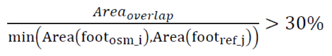
If the statement above is true, then the two building objects match, if not then they do not match.
On the other hand, the OSM community on the Talk-us mailing list, which included academics, discussed a slightly different equation. Instead of dividing by the smallest area (either footosm_i or footref_j), they used the PostGIS function ST_Area(ST_Union(footosm_i, footref_j)).
Assess Matches
With all the building footprints matched, the following metrics can be calculated. Exact methods to measure each metric will be determined. Refer to the Literature Review to see how these metrics are evaluated: (i) semantic accuracy, (ii) positional accuracy, (iii) size accuracy, (iv) shape accuracy, (v) attribute accuracy.
From the results of each assessment, different thresholds will be assigned to determine the quality of each OSM building (e.g., if the centroid distance between a matched OSM polygon and reference polygon is less than 0.2m, we can consider the quality of the OSM polygon to be “great”).
Work Cited
Avbelji, Janja, Rupert Müller, Richard Bamler, “A Metric for Polygon Comparison and Building Extraction Evaluation,” Geoscience and Remote Sensing Letters 12, no. 1 (2015): 1-5.
Arkin, M. Esther, L. Paul Chew, Daniel P. Huttenlocher, Klara Kedem, and Joseph S. B. Mitchell, “An Efficiently Computable Metric for Comparing Polygonal Shapes,” IEEE Transactions on Pattern Analysis and Machine Intelligence 13, no. 3 (1991): 209-216.
Brovelli, M. A., M. Minghini, M. E. Molinari, G. Zamboni, “Positional accuracy assessment of the OpenStreetMap buildings layer through automatic homologous pairs detection: the method and a case study,” The International Archives of the Photogrammetry, Remote Sensing and Spatial Information Sciences XLI-B2 (2016): 12-19.
Ciepluch, B., P. Mooney, A. Winstanley, “Building Generic Quality Indicators for OpenStreetMap.” Paper presented at the 19th Annual GIS Research UK (GISRUK), 2011.
Fan, Hongchao and Alexander Zipf, “Quality assessment for building footprints data on OpenStreetMap,” International Journal of Geographical Information Science 28, no. 4 (2014): 700-719.
Girres, Jean-Francois and Guillaume Touya, “Elements of quality assessment of French OpenStreetMap data,” Transactions in GIS 14, no. 4 (2010): 435-459.
Li, Wenwen, Michael F. Goodchild, Richard L. Church, “An Efficient Measure of Compactness for 2D Shapes and its Application in Regionalization Problems,” International Journal of Geographical Information Science (2013): 1-24.
Haklay, Mordechai, “How good is volunteered geographic information? A comparative study of OpenStreetMap and Ordnance Survey datasets,” Environment and Planning B: Planning and Design 37 (2010): 682-703. doi:10.1068/b35097.
Hechet, Robert, Carola Kunze, and Stefan Hahmann, “Measuring Completeness of Building Footprints in OpenStreetMap over Space and Time,” ISPRS International Journal of Geo-Information 2 (2013): 1066-1091. doi:10.3390/ijgi2041066.
Höpfner, S., “Vergleich der Adressdatensätze OpenAddresses, OpenStreetMap und TeleAtlas,” Bachelor Thesis, TU Dresden, Germany, 2011.
Ludwig, I., A. Voss, M. Krause-Traudes, “A Comparison of the Street Networks of Navteq and OSM in Germany,” in Advancing Geoinformation Science for a Changing World, ed. S. Geertman, W. Reinhardt, F. Toppen (Berlin, Germany: Springer, 2011), 65-84.
Neis, P., D. Zielstra, A. Zipf, “The street network evolution of crowdsourced maps: OpenStreetMap in Germany 2007-2011, Future Internet 4 (2011): 1-21.
Osserman, R., “Isoperimetric inequality,” Bulletin of the American Mathematical Society 84, no. 6 (1978): 1182-1238.
Maceachren, Alan M., “Compactness of Geographic Shape: Comparison and Evaluation of Measures,” Geografiska Annaler 67, no. 1 (1985): 53-67.
Miller, V. C., “A Quantitative Geomorphic Study of Drainage Basin Characteristics in the Clinch Mountain Area, Virginia and Tennessee,” Technical Report No. 3, Columbia University, New York, 1953.
Mooney P., P. Corcoran, A. Winstanley, “Towards quality metrics for OpenStreetMap.” Paper presented at the 18th SIGSPATIAL International Conference on Advances in Geographic Information Systems, San Jose, USA, November 2-5, 2010.
Müller, Fabian, Ionut Iosifescu, and Lorenz Hurni, “Assessment and Visualization of OSM Building Footprint Quality.” Paper presented at the 27th International Cartographic Conference, Rio de Janeiro, Brazil, August 23-28, 2015.
Rutzinger, M., F. Rottensteiner, N. Pfeifer, “A Comparison of Evaluation Techniques for Building Extraction From Airborne Laser Scanning,” IEEE Journal of Selected Topics in Applied Earth Observations and Remote Sensing 2, no. 1: 11-20.
Sehra, Sukhjit Singh, Jaiteg Singh, Hardeep Singh Rai, “Assessing OpenStreetMap Data Using Intrinsic Quality Indicators: An Extension to the QGIS Processing Toolbox,” Future Internet 9, no. 15 (2017): 1-22. doi:10.3390/fi9020015.
Zielstra, D., A. Zipf, “A Comparative Study of Proprietary Geodata and Volunteered Geographic Information for Germany.” Paper presented at the 13th International Conference on Geographic Information Science, Guimaraes, Portugal, May 10-14, 2010.